多层感知机实现:基于MNIST手写数字识别
目录
一、概述
二、网络架构设计
三、算法实现细节
1、依赖库导入
2、神经网络类构建
3、训练流程实现
4、参数矩阵初始化方法
5、矩阵与向量转换
6、梯度下降优化
6.1、损失函数计算
6.1.1、前向传播过程
6.2、反向传播算法
7、预测功能实现
四、完整代码实现
五、MNIST手写数字识别应用
一、概述
本文将详细介绍如何构建一个完整的多层感知机网络,并通过MNIST手写数字数据集进行验证。读者应具备神经网络基础知识,包括前向传播、反向传播、激活函数等概念。
我们将实现一个三层神经网络,通过784个输入特征(28×28像素图像)识别0-9的手写数字,并在测试集上评估模型性能。
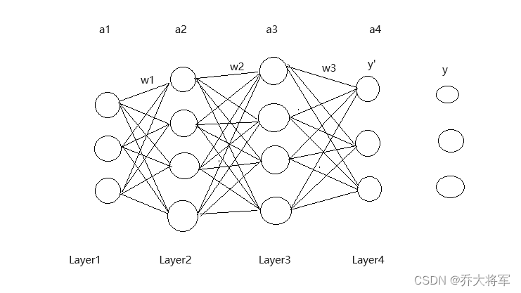
二、网络架构设计
网络采用三层结构:
- 输入层:784个神经元(对应28×28像素)
- 隐藏层:25个神经元
- 输出层:10个神经元(对应0-9数字)
关键设计考虑:
- 输入数据为784维特征向量
- 权重矩阵维度设计
- 前向传播计算流程
- Sigmoid激活函数应用
- 反向传播误差计算
- 偏置项处理
- 损失函数定义
- 权重更新规则
反向传播误差计算公式:
δ(4) = a(4) - y
δ(3) = (Θ³)ᵀδ(4) * g'(z³)
δ(2) = (Θ²)ᵀδ(3) * g'(z²)
δ(1) = 输入层,不可更新
g'为Sigmoid梯度函数
g'(z) = g(z)(1-g(z)); 其中g(z) = 1/(1+e⁻ᶻ)
梯度下降算法流程:
for i=1 to m
  设置a(1)=x⁽ⁱ⁾
  执行前向传播计算各层a⁽ˡ⁾, l=2,3...L
  使用y⁽ⁱ⁾计算δ(L)=a⁽ᴸ⁾-y⁽ⁱ⁾
  计算δ(L-1), δ(L-2)...δ(2)
  更新Δ⁽ˡ⁽ᵢⱼ⁾⁾: Δ⁽ˡ⁽ᵢⱼ⁾⁾ += a⁽ˡ⁾ⱼδ⁽ˡ⁺¹⁾ᵢ
三、算法实现细节
1、依赖库导入
import numpy as np
from Neural_Network_Lab.utils.features import prepare_for_training
from Neural_Network_Lab.utils.hypothesis import sigmoid, sigmoid_gradient
工具函数模块封装了数据预处理和激活函数实现。
2、神经网络类构建
class NeuralNetwork:
    def __init__(self, data, labels, layers, normalize_data=False):
        data_processed = prepare_for_training(data, normalize_data=normalize_data)[0]
        self.data = data_processed
        self.labels = labels
        self.layers = layers  # [784, 25, 10]
        self.normalize_data = normalize_data
        self.weights = NeuralNetwork.initialize_weights(layers)
3、训练流程实现
    def train(self, max_iterations=1000, learning_rate=0.1):
        # 将权重矩阵转换为向量便于优化
        flattened_weights = NeuralNetwork.flatten_weights(self.weights)
        optimized_weights, cost_history = NeuralNetwork.gradient_descent(
            self.data, self.labels, flattened_weights, self.layers,
            max_iterations, learning_rate
        )
        self.weights = NeuralNetwork.reshape_weights(optimized_weights, self.layers)
        return self.weights, cost_history
4、参数矩阵初始化方法
    @staticmethod
    def initialize_weights(layers):
        num_layers = len(layers)
        weights = {}  # 使用字典存储各层权重
        for layer_idx in range(num_layers - 1):
            input_count = layers[layer_idx]
            output_count = layers[layer_idx + 1]
            # 初始化小随机值,考虑偏置项
            weights[layer_idx] = np.random.rand(output_count, input_count + 1) * 0.05
        return weights
5、矩阵与向量转换
    @staticmethod
    def flatten_weights(weights):
        num_weight_layers = len(weights)
        flattened = np.array([])
        for layer_idx in range(num_weight_layers):
            flattened = np.hstack((flattened, weights[layer_idx].flatten()))
        return flattened

    @staticmethod
    def reshape_weights(flattened, layers):
        num_layers = len(layers)
        weights = {}
        shift = 0
        for layer_idx in range(num_layers - 1):
            input_count = layers[layer_idx]
            output_count = layers[layer_idx + 1]

            width = input_count + 1
            height = output_count
            volume = width * height

            start_idx = shift
            end_idx = shift + volume
            layer_flattened = flattened[start_idx:end_idx]
            weights[layer_idx] = layer_flattened.reshape((height, width))
            shift += volume

        return weights
6、梯度下降优化
6.1、损失函数计算
6.1.1、前向传播过程
    @staticmethod
    def forward_propagation(data, weights, layers):
        num_layers = len(layers)
        num_examples = data.shape[0]
        current_activation = data  # 输入层激活值

        # 逐层计算
        for layer_idx in range(num_layers - 1):
            weight = weights[layer_idx]
            next_activation = sigmoid(np.dot(current_activation, weight.T))
            # 添加偏置项
            next_activation = np.hstack((np.ones((num_examples, 1)), next_activation))
            current_activation = next_activation

        # 返回输出层结果(不含偏置项)
        return current_activation[:, 1:]
损失函数实现:
    @staticmethod
    def calculate_cost(data, labels, weights, layers):
        num_layers = len(layers)
        num_examples = data.shape[0]
        num_labels = layers[-1]

        # 前向传播获取预测结果
        predictions = NeuralNetwork.forward_propagation(data, weights, layers)

        # 创建one-hot编码标签
        one_hot_labels = np.zeros((num_examples, num_labels))
        for example_idx in range(num_examples):
            one_hot_labels[example_idx][labels[example_idx][0]] = 1

        # 计算交叉熵损失
        correct_cost = np.sum(np.log(predictions[one_hot_labels == 1]))
        incorrect_cost = np.sum(np.log(1 - predictions[one_hot_labels == 0]))
        cost = (-1/num_examples) * (correct_cost + incorrect_cost)
        return cost
6.2、反向传播算法
    @staticmethod
    def backpropagation(data, labels, weights, layers):
        num_layers = len(layers)
        (num_examples, num_features) = data.shape
        num_classes = layers[-1]

        # 初始化误差项
        errors = {}
        for layer_idx in range(num_layers - 1):
            input_count = layers[layer_idx]
            output_count = layers[layer_idx + 1]
            errors[layer_idx] = np.zeros((output_count, input_count + 1))

        # 对每个样本计算误差
        for example_idx in range(num_examples):
            layer_inputs = {}
            layer_activations = {}
            activation = data[example_idx, :].reshape((num_features, 1))
            layer_activations[0] = activation

            # 前向传播记录中间值
            for layer_idx in range(num_layers - 1):
                weight = weights[layer_idx]
                layer_input = np.dot(weight, activation)
                activation = np.vstack((np.array([[1]]), sigmoid(layer_input)))
                layer_inputs[layer_idx + 1] = layer_input
                layer_activations[layer_idx + 1] = activation

            output_activation = activation[1:, :]

            # 计算输出层误差
            delta = {}
            one_hot_label = np.zeros((num_classes, 1))
            one_hot_label[labels[example_idx][0]] = 1
            delta[num_layers - 1] = output_activation - one_hot_label

            # 反向计算各层误差
            for layer_idx in range(num_layers - 2, 0, -1):
                weight = weights[layer_idx]
                next_delta = delta[layer_idx + 1]
                layer_input = layer_inputs[layer_idx]
                layer_input = np.vstack((np.array([1]), layer_input))
                delta[layer_idx] = np.dot(weight.T, next_delta) * sigmoid(layer_input)
                delta[layer_idx] = delta[layer_idx][1:, :]

            # 累加梯度
            for layer_idx in range(num_layers - 1):
                layer_error = np.dot(delta[layer_idx + 1], layer_activations[layer_idx].T)
                errors[layer_idx] = errors[layer_idx] + layer_error

        # 平均梯度
        for layer_idx in range(num_layers - 1):
            errors[layer_idx] = errors[layer_idx] * (1/num_examples)

        return errors
梯度下降步骤实现:
    @staticmethod
    def gradient_step(data, labels, current_weights, layers):
        weights = NeuralNetwork.reshape_weights(current_weights, layers)
        gradients = NeuralNetwork.backpropagation(data, labels, weights, layers)
        flattened_gradients = NeuralNetwork.flatten_weights(gradients)
        return flattened_gradients

    @staticmethod
    def gradient_descent(data, labels, initial_weights, layers, max_iterations, learning_rate):
        optimized_weights = initial_weights
        cost_history = []

        for iteration in range(max_iterations):
            if iteration % 10 == 0:
                print(f"当前迭代次数: {iteration}")

            cost = NeuralNetwork.calculate_cost(
                data, labels,
                NeuralNetwork.reshape_weights(optimized_weights, layers),
                layers
            )
            cost_history.append(cost)

            gradients = NeuralNetwork.gradient_step(data, labels, optimized_weights, layers)
            optimized_weights = optimized_weights - learning_rate * gradients

        return optimized_weights, cost_history
7、预测功能实现
    def predict(self, data):
        data_processed = prepare_for_training(data, normalize_data=self.normalize_data)[0]
        num_examples = data_processed.shape[0]
        predictions = NeuralNetwork.forward_propagation(data_processed, self.weights, self.layers)

        return np.argmax(predictions, axis=1).reshape((num_examples, 1))
四、完整代码实现
import numpy as np
from Neural_Network_Lab.utils.features import prepare_for_training
from Neural_Network_Lab.utils.hypothesis import sigmoid, sigmoid_gradient

class NeuralNetwork:
    def __init__(self, data, labels, layers, normalize_data=False):
        data_processed = prepare_for_training(data, normalize_data=normalize_data)[0]
        self.data = data_processed
        self.labels = labels
        self.layers = layers  # [784, 25, 10]
        self.normalize_data = normalize_data
        self.weights = NeuralNetwork.initialize_weights(layers)

    def predict(self, data):
        data_processed = prepare_for_training(data, normalize_data=self.normalize_data)[0]
        num_examples = data_processed.shape[0]
        predictions = NeuralNetwork.forward_propagation(data_processed, self.weights, self.layers)

        return np.argmax(predictions, axis=1).reshape((num_examples, 1))

    def train(self, max_iterations=1000, learning_rate=0.1):
        flattened_weights = NeuralNetwork.flatten_weights(self.weights)
        optimized_weights, cost_history = NeuralNetwork.gradient_descent(
            self.data, self.labels, flattened_weights, self.layers,
            max_iterations, learning_rate
        )
        self.weights = NeuralNetwork.reshape_weights(optimized_weights, self.layers)
        return self.weights, cost_history

    @staticmethod
    def gradient_descent(data, labels, initial_weights, layers, max_iterations, learning_rate):
        optimized_weights = initial_weights
        cost_history = []

        for iteration in range(max_iterations):
            if iteration % 10 == 0:
                print(f"当前迭代次数: {iteration}")

            cost = NeuralNetwork.calculate_cost(
                data, labels,
                NeuralNetwork.reshape_weights(optimized_weights, layers),
                layers
            )
            cost_history.append(cost)

            gradients = NeuralNetwork.gradient_step(data, labels, optimized_weights, layers)
            optimized_weights = optimized_weights - learning_rate * gradients

        return optimized_weights, cost_history

    @staticmethod
    def gradient_step(data, labels, current_weights, layers):
        weights = NeuralNetwork.reshape_weights(current_weights, layers)
        gradients = NeuralNetwork.backpropagation(data, labels, weights, layers)
        flattened_gradients = NeuralNetwork.flatten_weights(gradients)
        return flattened_gradients

    @staticmethod
    def backpropagation(data, labels, weights, layers):
        num_layers = len(layers)
        (num_examples, num_features) = data.shape
        num_classes = layers[-1]

        errors = {}
        for layer_idx in range(num_layers - 1):
            input_count = layers[layer_idx]
            output_count = layers[layer_idx + 1]
            errors[layer_idx] = np.zeros((output_count, input_count + 1))

        for example_idx in range(num_examples):
            layer_inputs = {}
            layer_activations = {}
            activation = data[example_idx, :].reshape((num_features, 1))
            layer_activations[0] = activation

            for layer_idx in range(num_layers - 1):
                weight = weights[layer_idx]
                layer_input = np.dot(weight, activation)
                activation = np.vstack((np.array([[1]]), sigmoid(layer_input)))
                layer_inputs[layer_idx + 1] = layer_input
                layer_activations[layer_idx + 1] = activation

            output_activation = activation[1:, :]

            delta = {}
            one_hot_label = np.zeros((num_classes, 1))
            one_hot_label[labels[example_idx][0]] = 1
            delta[num_layers - 1] = output_activation - one_hot_label

            for layer_idx in range(num_layers - 2, 0, -1):
                weight = weights[layer_idx]
                next_delta = delta[layer_idx + 1]
                layer_input = layer_inputs[layer_idx]
                layer_input = np.vstack((np.array([1]), layer_input))
                delta[layer_idx] = np.dot(weight.T, next_delta) * sigmoid(layer_input)
                delta[layer_idx] = delta[layer_idx][1:, :]

            for layer_idx in range(num_layers - 1):
                layer_error = np.dot(delta[layer_idx + 1], layer_activations[layer_idx].T)
                errors[layer_idx] = errors[layer_idx] + layer_error

        for layer_idx in range(num_layers - 1):
            errors[layer_idx] = errors[layer_idx] * (1/num_examples)

        return errors

    @staticmethod
    def calculate_cost(data, labels, weights, layers):
        num_layers = len(layers)
        num_examples = data.shape[0]
        num_labels = layers[-1]

        predictions = NeuralNetwork.forward_propagation(data, weights, layers)

        one_hot_labels = np.zeros((num_examples, num_labels))
        for example_idx in range(num_examples):
            one_hot_labels[example_idx][labels[example_idx][0]] = 1

        correct_cost = np.sum(np.log(predictions[one_hot_labels == 1]))
        incorrect_cost = np.sum(np.log(1 - predictions[one_hot_labels == 0]))
        cost = (-1/num_examples) * (correct_cost + incorrect_cost)
        return cost

    @staticmethod
    def forward_propagation(data, weights, layers):
        num_layers = len(layers)
        num_examples = data.shape[0]
        current_activation = data

        for layer_idx in range(num_layers - 1):
            weight = weights[layer_idx]
            next_activation = sigmoid(np.dot(current_activation, weight.T))
            next_activation = np.hstack((np.ones((num_examples, 1)), next_activation))
            current_activation = next_activation

        return current_activation[:, 1:]

    @staticmethod
    def reshape_weights(flattened, layers):
        num_layers = len(layers)
        weights = {}
        shift = 0
        for layer_idx in range(num_layers - 1):
            input_count = layers[layer_idx]
            output_count = layers[layer_idx + 1]

            width = input_count + 1
            height = output_count
            volume = width * height

            start_idx = shift
            end_idx = shift + volume
            layer_flattened = flattened[start_idx:end_idx]
            weights[layer_idx] = layer_flattened.reshape((height, width))
            shift += volume

        return weights

    @staticmethod
    def flatten_weights(weights):
        num_weight_layers = len(weights)
        flattened = np.array([])
        for layer_idx in range(num_weight_layers):
            flattened = np.hstack((flattened, weights[layer_idx].flatten()))
        return flattened

    @staticmethod
    def initialize_weights(layers):
        num_layers = len(layers)
        weights = {}
        for layer_idx in range(num_layers - 1):
            input_count = layers[layer_idx]
            output_count = layers[layer_idx + 1]
            weights[layer_idx] = np.random.rand(output_count, input_count + 1) * 0.05
        return weights
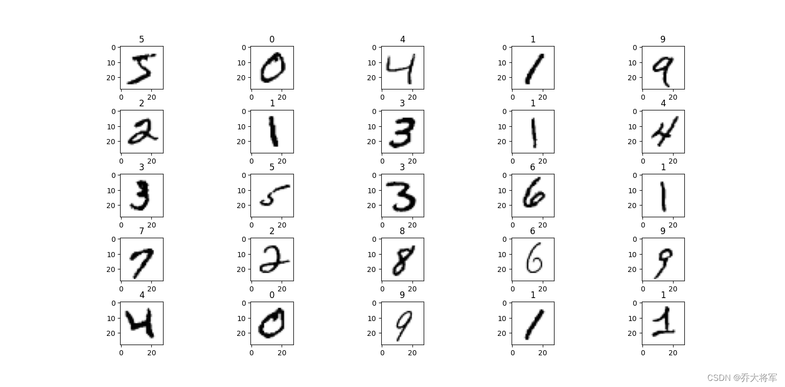
五、MNIST手写数字识别应用
MNIST数据集包含10,000个手写数字样本,每张图像为28×28像素,第一列为标签,其余784列为像素值。
import numpy as np
import pandas as pd
import matplotlib.pyplot as plt
import math
from Neural_Network_Lab.Neural_Network import NeuralNetwork
# 加载数据
data = pd.read_csv('../Neural_Network_Lab/data/mnist-demo.csv')
# 可视化部分样本
num_samples = 25
grid_size = math.ceil(math.sqrt(num_samples))
plt.figure(figsize=(10, 10))
for plot_idx in range(num_samples):
digit = data[plot_idx:plot_idx+1].values
label = digit[0][0]
pixels = digit[0][1:]
image_size = int(math.sqrt(pixels.shape[0]))
image = pixels.reshape((image_size, image_size))
plt.subplot(grid_size, grid_size, plot_idx+1)
plt.imshow(image, cmap='Greys')
plt.title(label)
plt.subplots_adjust(wspace=0.5, hspace=0.5)
plt.show()
# 划分训练集和测试集
train_data = data.sample(frac=0.8)
test_data = data.drop(train_data.index)
train_data = train_data.values
test_data = test_data.values
num_training_samples = 8000
X_train = train_data[:num_training_samples, 1:]
y_train = train_data[:num_training_samples, [0]]
X_test = test_data[:, 1:]
y_test = test_data[:, [0]]
# 设置网络参数
layers = [784, 25, 10]
normalize_data = True
max_iterations = 500
learning_rate = 0.1
# 创建并训练神经网络
nn = NeuralNetwork(X_train, y_train, layers, normalize_data)
(weights, cost_history) = nn.train(max_iterations, learning_rate)
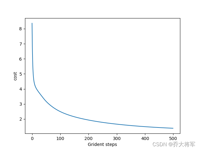
# 绘制损失曲线
plt.plot(range(len(cost_history)), cost_history)
plt.xlabel('迭代次数')
plt.ylabel('损失值')
plt.show()
# 进行预测
train_predictions = nn.predict(X_train)
test_predictions = nn.predict(X_test)
# 计算准确率
train_accuracy = np.sum((train_predictions == y_train) / y_train.shape[0] * 100)
test_accuracy = np.sum((test_predictions == y_test) / y_test.shape[0] * 100)
print(f"训练集准确率: {train_accuracy:.2f}%")
print(f"测试集准确率: {test_accuracy:.2f}%")
# 可视化预测结果
num_samples = 64
grid_size = math.ceil(math.sqrt(num_samples))
plt.figure(figsize=(15, 15))
for plot_idx in range(num_samples):
true_label = y_test[plot_idx, 0]
pixels = X_test[plot_idx, :]
predicted_label = test_predictions[plot_idx][0]
image_size = int(math.sqrt(pixels.shape[0]))
image = pixels.reshape((image_size, image_size))
plt.subplot(grid_size, grid_size, plot_idx+1)
color_map = 'Greens' if predicted_label == true_label else 'Reds'
plt.imshow(image, cmap=color_map)
plt.title(predicted_label)
plt.tick_params(axis='both', which='both', bottom=False, left=False, labelbottom=False)
plt.subplots_adjust(wspace=0.5, hspace=0.5)
plt.show()
实验使用8,000个样本进行训练,2,000个样本进行测试,迭代500次。
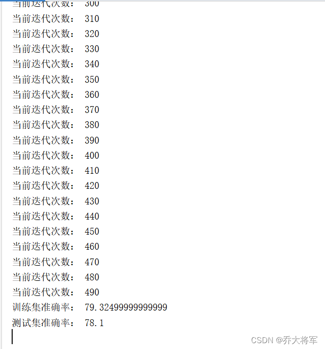
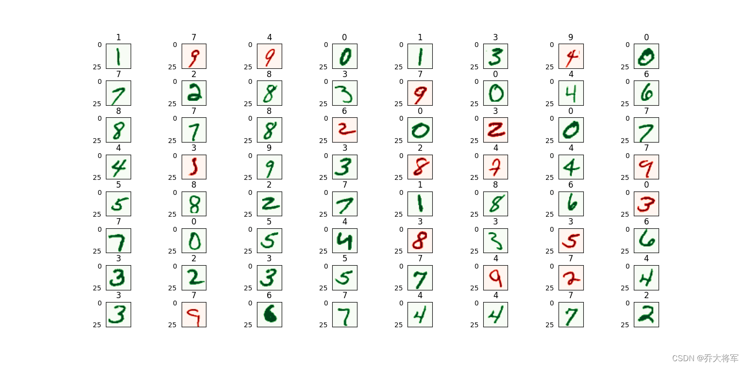
当前模型准确率有待提高,读者可通过调整迭代次数、网络层次或增加训练数据来提升性能。
