基于梯度下降的逻辑回归分类模型实现
项目背景与目标
本任务旨在构建一个逻辑回归分类器,用于预测学生是否能被大学录取。作为招生管理部门的一员,我们需要根据申请者在两门入学考试中的成绩来评估其录取概率。历史数据包含100名学生的考试分数及最终录取结果(1表示录取,0表示未录取)。我们将利用这些数据训练模型,并通过优化算法求解参数。
数据加载与可视化
import numpy as np
import pandas as pd
import matplotlib.pyplot as plt

# 加载数据
file_path = 'data/LogiReg_data.txt'
data_frame = pd.read_csv(file_path, header=None, names=['Exam1', 'Exam2', 'Admitted'])
data_frame.head()
| Exam1 | Exam2 | Admitted | |
|---|---|---|---|
| 0 | 34.623660 | 78.024693 | 0 |
| 1 | 30.286711 | 43.894998 | 0 |
| 2 | 35.847409 | 72.902198 | 0 |
| 3 | 60.182599 | 86.308552 | 1 |
| 4 | 79.032736 | 75.344376 | 1 |
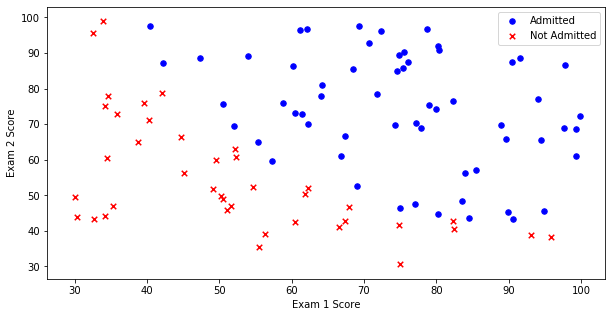
数据集共包含100条记录和3个特征列。接下来对样本进行可视化:
admitted_group = data_frame[data_frame['Admitted'] == 1]
not_admitted_group = data_frame[data_frame['Admitted'] == 0]

fig, axis = plt.subplots(figsize=(10, 5))
axis.scatter(admitted_group['Exam1'], admitted_group['Exam2'], c='blue', marker='o', label='录取', s=30)
axis.scatter(not_admitted_group['Exam1'], not_admitted_group['Exam2'], c='red', marker='x', label='未录取', s=30)
axis.set_xlabel('考试1成绩')
axis.set_ylabel('考试2成绩')
axis.legend()
核心组件设计
为完成逻辑回归建模,需实现以下关键函数:
logit:将线性输出映射至[0,1]区间的激活函数predict_proba:前向传播计算预测概率compute_loss:交叉熵损失函数calculate_gradient:参数梯度计算update_params:执行参数更新步骤evaluate_accuracy:模型准确率评估
S形激活函数
定义Sigmoid函数将实数域映射到(0,1)区间,解释为正类发生的概率:
\[ \sigma(z) = \frac{1}{1 + e^{-z}} \]def logit(z):
return 1 / (1 + np.exp(-np.clip(z, -250, 250))) # 防止溢出
# 可视化函数形态
inputs = np.linspace(-10, 10, 100)
outputs = logit(inputs)
plt.plot(inputs, outputs, 'g-', linewidth=2)
plt.title('Sigmoid Function')
plt.grid(True)
模型预测函数
构造增广矩阵并计算线性组合:
\[ X\theta^T = \begin{bmatrix} 1 & x_1^{(1)} & x_2^{(1)} \\ \vdots & \vdots & \vdots \\ 1 & x_1^{(m)} & x_2^{(m)} \end{bmatrix} \begin{bmatrix} \theta_0 \\ \theta_1 \\ \theta_2 \end{bmatrix} \]# 添加偏置项
data_frame.insert(0, 'Bias', 1)
raw_array = data_frame.values
num_features = raw_array.shape[1]
X_train = raw_array[:, 0:num_features-1]
y_target = raw_array[:, num_features-1:num_features]
params = np.zeros((1, X_train.shape[1]))
def predict_proba(X, weights):
z = X @ weights.T
return logit(z)
损失函数定义
采用对数似然的负值作为代价函数:
\[ J(\theta) = -\frac{1}{m} \sum_{i=1}^{m} \left[ y^{(i)}\log(\hat{y}^{(i)}) + (1-y^{(i)})\log(1-\hat{y}^{(i)}) \right] \]def compute_loss(X, y, weights):
m = len(X)
preds = predict_proba(X, weights).ravel()
# 添加数值稳定性处理
preds = np.clip(preds, 1e-15, 1 - 1e-15)
loss = -np.mean(y.ravel() * np.log(preds) + (1 - y.ravel()) * np.log(1 - preds))
return loss
梯度计算
对每个参数求偏导:
\[ \frac{\partial J}{\partial \theta_j} = \frac{1}{m} \sum_{i=1}^{m} (\hat{y}^{(i)} - y^{(i)}) x_j^{(i)} \]def calculate_gradient(X, y, weights):
m = len(X)
error = (predict_proba(X, weights) - y).ravel()
grad = np.empty(weights.shape[1])
for j in range(weights.shape[1]):
grad[j] = np.dot(error, X[:, j]) / m
return grad.reshape(1, -1)
优化策略对比
实现三种梯度下降变体:
ITERATION_STOP = 0
LOSS_STOP = 1
GRADIENT_STOP = 2

def should_stop(criterion_type, current_value, threshold):
    if criterion_type == ITERATION_STOP:
        return current_value > threshold
    elif criterion_type == LOSS_STOP:
        return abs(current_value[-1] - current_value[-2]) < threshold
    else:
        return np.linalg.norm(current_value) < threshold

def shuffle_dataset(arr):
    np.random.shuffle(arr)
    cols = arr.shape[1]
    return arr[:, :-1], arr[:, -1:]

def update_params(data, init_weights, batch_size, stop_mode, limit, lr_rate):
    start_time = time.time()
    epoch_count = 0
    batch_idx = 0
    X_src, y_src = shuffle_dataset(data)
    current_w = init_weights.copy()
    losses = [compute_loss(X_src, y_src, current_w)]

    while True:
        X_batch = X_src[batch_idx: batch_idx + batch_size]
        y_batch = y_src[batch_idx: batch_idx + batch_size]

        grad_vector = calculate_gradient(X_batch, y_batch, current_w)
        current_w -= lr_rate * grad_vector

        batch_idx += batch_size
        if batch_idx >= len(data):
            batch_idx = 0
            X_src, y_src = shuffle_dataset(data)

        new_loss = compute_loss(X_src, y_src, current_w)
        losses.append(new_loss)
        epoch_count += 1

        if stop_mode == ITERATION_STOP:
            check_val = epoch_count
        elif stop_mode == LOSS_STOP:
            check_val = losses
        else:
            check_val = grad_vector

        if should_stop(stop_mode, check_val, limit):
            break

    elapsed = time.time() - start_time
    return current_w, epoch_count, losses, elapsed
不同停止条件实验
固定迭代次数(5000轮):
n_samples = len(orig_data)
final_weights, epochs, loss_history, duration = update_params(
    orig_data, params, n_samples, ITERATION_STOP, 5000, 1e-6)
print(f"耗时: {duration:.2f}s, 最终损失: {loss_history[-1]:.3f}")
基于损失变化量停止(阈值1e-6):
_, _, _, _ = update_params(orig_data, params, n_samples, LOSS_STOP, 1e-6, 1e-3)
基于梯度范数停止(阈值0.05):
_, _, _, _ = update_params(orig_data, params, n_samples, GRADIENT_STOP, 0.05, 1e-3)
批量策略比较
随机梯度下降(SGD):
run_experiment(orig_data, params, 1, ITERATION_STOP, 5000, 0.001)
小批量梯度下降(Mini-batch):
run_experiment(orig_data, params, 16, ITERATION_STOP, 15000, 0.001)
数据标准化提升性能
使用 sklearn 对输入特征进行归一化处理:
from sklearn.preprocessing import StandardScaler

processed_data = orig_data.copy()
scaler = StandardScaler()
processed_data[:, 1:3] = scaler.fit_transform(orig_data[:, 1:3])

# 在标准化数据上重新训练
optimal_params = run_experiment(processed_data, params, n_samples, GRADIENT_STOP, 0.02, 0.001)
模型评估
设定决策阈值为0.5进行分类:
def evaluate_accuracy(X, true_labels, learned_params):
    probas = predict_proba(X, learned_params)
    pred_labels = (probas >= 0.5).astype(int).ravel()
    accuracy_score = np.mean(pred_labels == true_labels.ravel())
    return accuracy_score

X_test = processed_data[:, :3]
y_true = processed_data[:, 3]
acc = evaluate_accuracy(X_test, y_true, optimal_params)
print(f'模型准确率: {acc*100:.1f}%')
